COMSOL has the best multiphysical simulation capabilities in my experience. Technical support from Elisa at TECHNIC as well as the engineers at COMSOL has been great.
COMSOL is an important part of our research in plasma physics. We use it in the design of plasma systems and it helps us to obtain a greater understanding of the underlying physics. We have always valued the quick support from TECHNIC and COMSOL and it has been a pleasure to work with them.
Comsol has become a valuable part of our design and decision making process. The exceptional flexibility and access to the physics and solvers in Comsol has allowed us to have deeper understanding on thermomechanical solutions. Technic and Comsol have always been quick and helpful to resolve any issues and provide helpful advice on their products.
At Scion we use COMSOL Multiphysics to understand energy processes, such as the interplay of non-linear solid mechanics and heat & mass transfer during biomass compaction, to design new or more efficient processes.
We use COMSOL Multiphysics to design the customised muffler. With it, we can simulate the insertion loss at different spectrum with different muffler designs.
Define and solve models for studying systems containing fluid flow and fluid flow coupled to other physical phenomena with the CFD Module, an add-on product to the COMSOL Multiphysics® simulation platform.
The CFD Module provides tools for modelling the cornerstones of fluid flow analysis, including:
These capabilities are implemented through structured fluid flow interfaces in order to define, solve, and analyse time-dependent (transient) and steady-state flow problems in 2D, 2D axisymmetry, and 3D. In addition to the list above, the CFD Module includes tailored functionality for solving problems that include non-Newtonian fluids, rotating machinery, and high Mach number flow.
The ability to implement multiphysics in a model is important for fluid flow analyses. With the CFD Module, you can model conjugate heat transfer and reacting flows in the same software environment you use to analyse fluid flow problems — simultaneously. Additional multiphysics possibilities, such as fluid-structure interaction, are available when combined with other modules within the COMSOL® product suite.
When you expand COMSOL Multiphysics® with the CFD Module, you have access to features for specialised CFD simulations in addition to the core functionality of the COMSOL Multiphysics® software platform. All of the features listed below are implemented through associated physics interfaces. When defining and solving these problems, the fluid is modelled as incompressible by default but can be interchanged with weakly compressible or fully compressible flow simply by choosing them from a list.
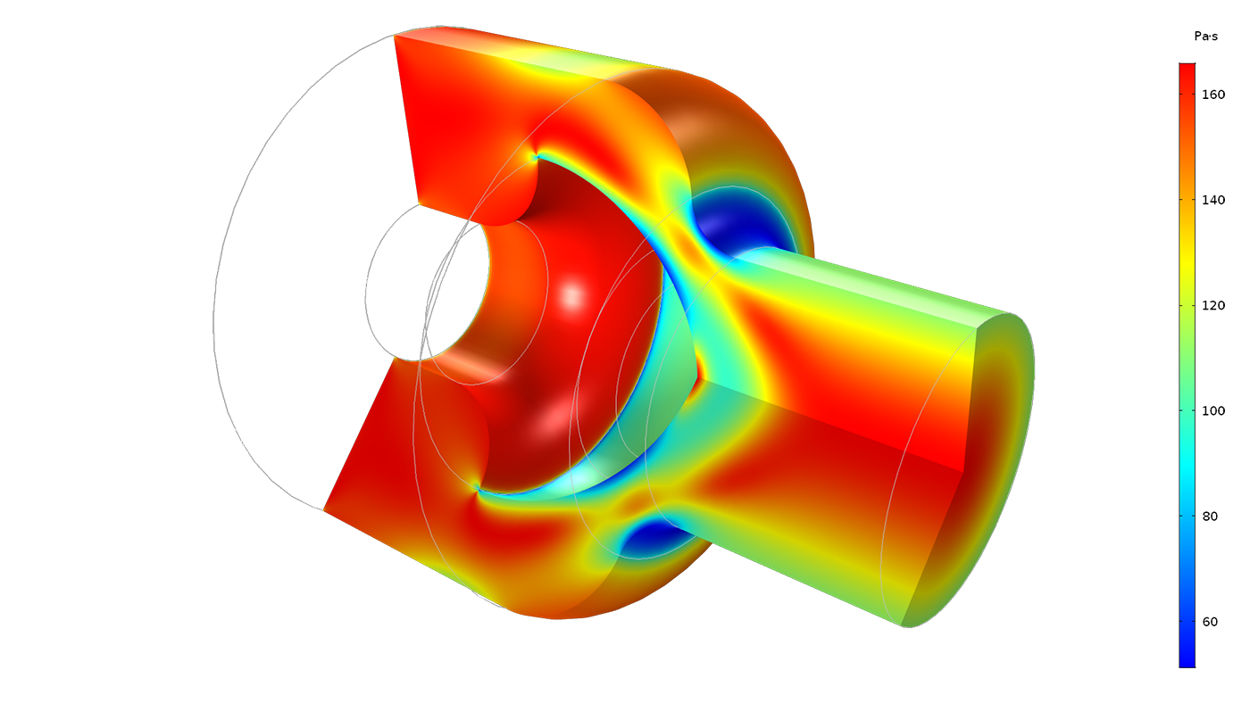
The Laminar Flow and Creeping Flow interfaces provide you with the functionality for modelling transient and steady flows at relatively low Reynolds numbers. A fluid viscosity may be dependent on the local composition and temperature or any other field that is modelled in combination with fluid flow. For non-Newtonian fluids, you can use the predefined rheology models for viscosity, such as Power Law, Carreau, and Bingham for easy model setup.
In general, density, viscosity, and momentum sources can be arbitrary functions of temperature, composition, shear rate, and any other dependent variable, as well as derivatives of dependent variables. These settings make it possible to define arbitrary models for viscoelastic flow.
A comprehensive set of Reynolds-averaged Navier-Stokes (RANS) turbulence models, as well as large eddy simulation, are available in the corresponding fluid flow interfaces in the CFD Module. The following turbulent flow models are available for transient and steady flows:
You can combine the turbulent flow interfaces with different types of wall treatments, according to the following list:
Change or extend the model equations directly in the graphical user interface (GUI) to create turbulence models that are not yet included.
To describe flows in thin domains, such as the thin oil films between moving mechanical parts or fractured structures, the CFD Module provides the Thin Film Flow, Shell interface. This formulation is typically used for modelling lubrication, elastohydrodynamics, or the effects of fluid damping between moving parts due to the presence of gases or liquids (for example, in MEMS).
The Thin Film Flow, Shell interface formulates and solves the Reynolds equation for flow in narrow structures and formulates the mass and momentum balances using a function for the flow averaged across the thickness of the thin structure, which implies that the thickness does not have to be meshed. This functionality helps avoid meshing problems across the gap and thereby saves computation time.
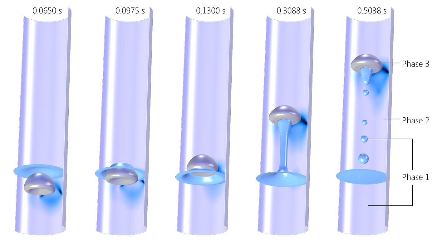
In separated multiphase flow systems, you can use surface tracking methods to model and simulate the behavior of bubbles and droplets in detail, as well as free surfaces. For such cases, the shape of the phase boundary can be described in detail, including surface tension effects, using surface tracking techniques for separated multiphase flow.
When bubbles, droplets, or particles are small compared to the computational domain and there is a large number of them, you can use dispersed multiphase flow models. These models keep track of the mass fraction of the different phases and the influence that the dispersed bubbles, droplets, or particles have on the transfer of momentum in the fluid in an averaged sense.
The following separated and dispersed multiphase flow models are available for transient and steady flows:
The CFD Module makes it simple to simulate fluid flow in porous media using three different porous media flow models.
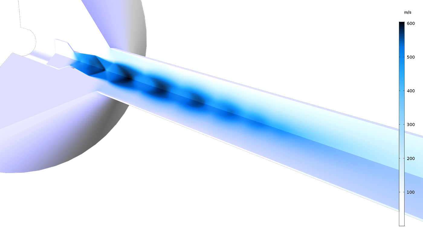
Model transonic and supersonic flows of compressible fluids in both laminar and turbulent regimes. The laminar flow model is typically used for low-pressure systems and automatically defines the equations for the momentum, mass, and energy balances for ideal gases. High Mach number flow is available for the k-ε and Spalart-Allmaras turbulence models.
The COMSOL® software automatically formulates the energy equation coupled to the momentum and mass balance equations for ideal gases. In both cases, when meshing these models, automatic mesh refinement resolves the shock pattern by refining around the regions with very high velocity and pressure gradients.
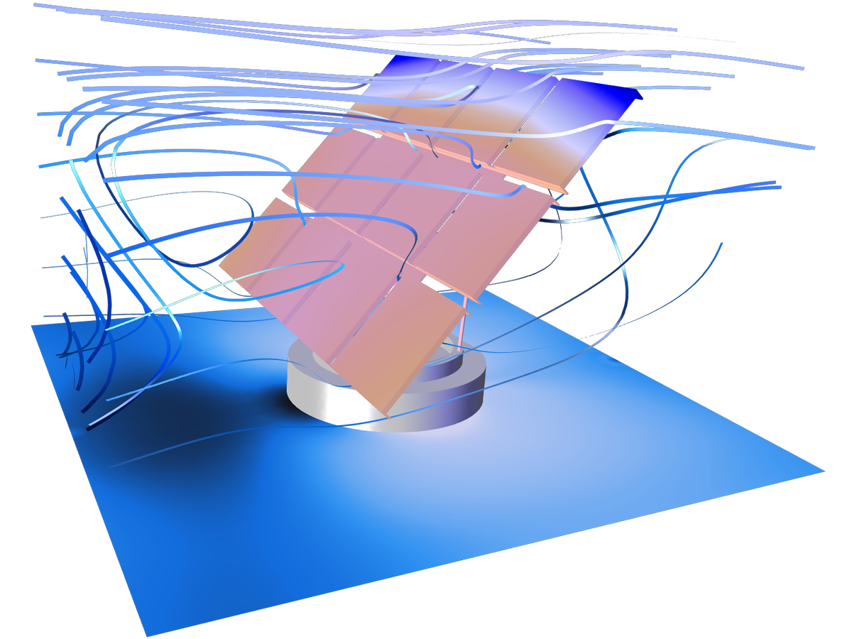
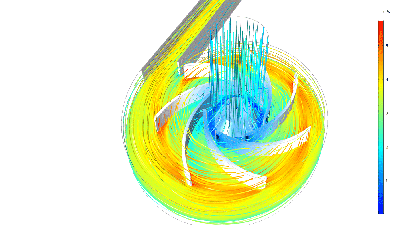
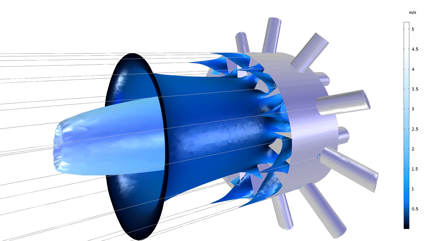
Rotating machines, such as mixers and pumps, are common in processes and equipment where fluid flow occurs. The CFD Module provides rotating machinery interfaces that formulate the fluid flow equations in rotating frames and are available for single-phase laminar and turbulent flow. Either define and solve problems using the full time-dependent description of the rotating system or use an averaged approach based on the frozen rotor approximation. This feature is computationally inexpensive and can be used to estimate averaged velocities, pressure changes, mixing levels, averaged temperature and concentration distributions, and more.
Generally speaking, the CFD Module can also solve fluid flow problems on any moving frame, not just rotating frames. You can use moving frames to solve a problem where a structure slides in relation to another structure with fluid flow in between, which is easy to set up and solve by employing a moving mesh.
In many cases, fluid flow models are coupled to other phenomena, such as heat transfer, structural mechanics, chemical reactions, or electromagnetic fields in electrokinetic flow and magnetohydrodynamics. Modelling multiple physics phenomena in COMSOL Multiphysics® is no different than a single-physics problem, as the CFD Module provides ready-made multiphysics interfaces for the common couplings.
In many cases, fluid flow models are coupled to other phenomena, such as heat transfer, structural mechanics, chemical reactions, or electromagnetic fields in electrokinetic flow and magnetohydrodynamics. Modelling multiple physics phenomena in COMSOL Multiphysics® is no different than a single-physics problem, as the CFD Module provides ready-made multiphysics interfaces for the common couplings.
The CFD Module provides a dedicated physics interface for defining models of heat transfer in fluid and solid domains coupled to fluid flow in the fluid domain. These types of models are denoted conjugate heat transfer models, which implies that the fluid flow equations are defined and solved in the fluid domain, while the heat transfer equations are formulated and solved in both the solid and fluid domains.
For laminar flows and turbulence models using the low-Reynolds-number wall treatment, the temperature is continuous across the solid-fluid internal boundary, which is the default setting in the nonisothermal flow interfaces. To simulate turbulent conjugate heat transfer using turbulence models with wall functions, the Nonisothermal Flow interface automatically defines thermal wall functions.
The options of low-Re formulations and thermal wall functions make it very straightforward to define and solve conjugate heat transfer problems in combination with turbulent flow.
With the addition of the Structural Mechanics Module, fluid-structure interaction (FSI) problems can be defined and solved for both laminar and turbulent flow. Two FSI options are available in the CFD Module:
The two-way coupling defines a moving mesh problem in the fluid domain. The displacements at the solid-fluid surfaces are determined by the balance of forces exerted by the fluid and counterforces exerted by the deforming solid structure. Steady-state and time-dependent studies are available for both one-way and two-way FSI problems for laminar and turbulent flows.
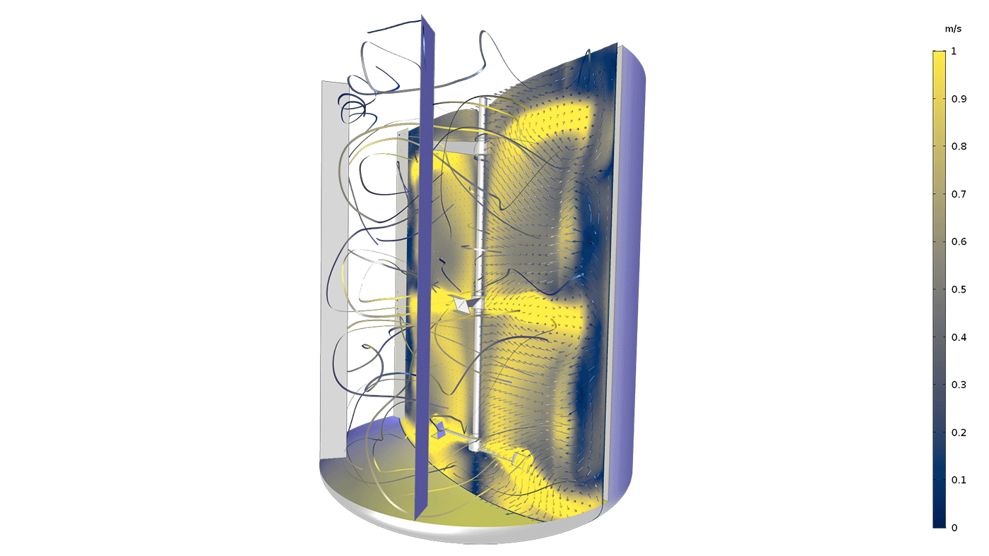
You can use the CFD Module to model reacting systems for both turbulent and laminar flows. This allows for the study and design of reactors, mixers, and any other system where chemical reactions and flow occur. The reacting flow interfaces are able to describe multicomponent transport in diluted and concentrated mixtures. The mixture-average model for multicomponent transport is used for concentrated solutions.
The full Maxwell-Stefan multicomponent transport equations are available in combination with the Chemical Reaction Engineering Module. For turbulent reacting flows, the eddy dissipation model is used to describe turbulence fluctuations in the reaction terms for both diluted and concentrated solutions. To simulate multicomponent transport in concentrated mixtures, the Stefan term is also automatically taken into account; for example, at reacting boundaries.
The Mixer Module expands the capabilities of the CFD Module by adding multiphase flow and free surfaces for rotating machinery. Additionally, you can access a Part Library for impellers and vessels to streamline geometry creation. Both of these features are well suited for modelling processes in the pharmaceutical and food industries.
The multiphase flow interfaces for dispersed flow in the CFD Module treat the dispersed phase as a field where its volume fraction is a model variable. When combined with the Particle Tracing Module, you can use the CFD Module to model Euler-Lagrange multiphase flow models, where particles or droplets are modelled as rigid particles. With rigid particles modelled separately, the interaction between the fluid and the particles is bidirectional, where the particles affect the fluid flow as well. In addition, the Euler-Lagrange models are computationally inexpensive when studying a relatively small volume fraction of particles.
The Pipe Flow Module defines models for networks of pipes and channels where the fluid flow equations can be solved along lines and curves. By combining this product with the CFD Module, you can create high-fidelity simulations that include pipes and channels connecting to 2D or 3D fluid domains with incompressible, weakly compressible, nonisothermal, and reacting flows.
When you build a simulation in COMSOL Multiphysics®, you follow a consistent workflow across all add-on modules. The CFD Module offers specialised functionality for fluid flow simulations to maximise the performance and accuracy you need for a CFD analysis. Here are a few of the CFD-specific features:
Generate flow domains, such as a bounding box, around imported CAD geometries. You can automatically or manually remove details included in a CAD representation that are not relevant for fluid flow.
The CFD Module includes a Material Library with the most common gases and liquids. In combination with the Chemical Reaction Engineering Module, you can also access generic descriptions for physical properties of gases (such as viscosity, density, diffusivities, and thermal conductivity).
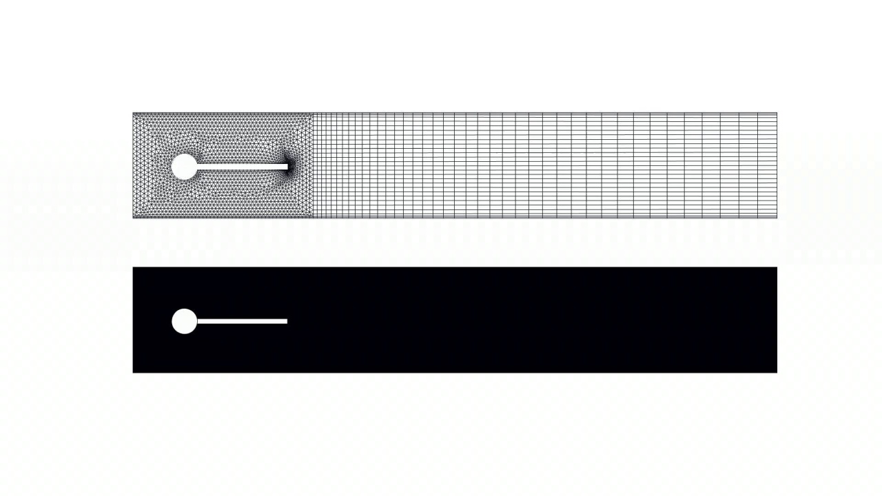
The physics-controlled mesh functionality in the CFD Module accounts for boundary conditions in fluid flow problems in order to compute accurate solutions. A boundary layer mesh is automatically generated in order to resolve the gradients in velocity that usually arise at the surfaces where wall conditions are applied.
The fluid flow physics interfaces use a Galerkin least-squares method to discretise the flow equations and generate the numerical model in space (2D, 2D axisymmetry, and 3D). The test function is designed to stabilise the hyperbolic terms and the pressure term in the transport equations. Shock-capturing techniques further reduce spurious oscillations. Additionally, discontinuous Galerkin formulations are used to conserve momentum, mass, and energy over internal and external boundaries.
The flow equations are usually highly nonlinear. In order to solve the numerical model equations, the automatic solver settings select a suitable damped Newton method. For large problems, the linear iterations in the Newton method are accelerated by state-of-the-art algebraic multigrid or geometric multigrid methods specifically designed for transport problems.
For transient problems, time-stepping techniques with automatic time stepping and automatic polynomial orders are used to resolve the velocity and pressure fields with the highest possible accuracy, in combination with the aforementioned nonlinear solvers.
The fluid flow interfaces generate a number of default plots to analyse the velocity and pressure fields. There is an extensive list of derived values and variables that can be easily accessed to extract analytical results.
You can build user interfaces on top of any existing model using the Application Builder, included in COMSOL Multiphysics®. This tool enables you to create applications for very specific purposes with well-defined inputs and outputs. Applications can be used for many different purposes:
In order to fully evaluate whether or not the COMSOL Multiphysics® software will meet your requirements, you need to contact us. By talking to one of our sales representatives, you will get personalised recommendations and fully documented examples to help you get the most out of your evaluation and guide you to choose the best license option to suit your needs.
Fill in your contact details and any specific comments or questions, and submit. You will receive a response from a sales representative within one business day.
 Tel: +61 (03) 6224 8690Email: info@technic.com.auConnect on LinkedInGet Your Free Trial
Copyright © 2021 Technic Pty Ltd. All Rights Reserved. See our Privacy Policy. Site protected by reCAPTCHA - Privacy | Terms. Website by Gloo.
